Audio Effects based on Biorthogonal Time-Varying Frequency Warping

Introduction

In audio signal processing, frequency warping describes the transformation of the spectral content of a sound via a mapping of the original set of frequencies to a new set of frequencies. If this mapping is linear, the original harmonics are scaled by some coefficient, resulting in a new harmonic structure. If it is nonlinear, the harmonic structure of some input periodic signal is ruined, resulting in an inharmonic set of partials. Inharmonicity can be wielded in many contexts. For example, it is well-known that low piano tones show inharmonicity. Therefore, frequency warping via a nonlinear map could be useful in digitally synthesizing piano sounds.

Another application of frequency warping via a nonlinear map is sound morphing. Given both the harmonic structure an input signal and a target signal, one can warp the frequency axis of the spectrum of the input signal over time to morph into the target signal.

A number of techniques for frequency warping are known. The most popular ones for musical applications include the present investigation (using a generalized Laguerre transform) described in [1], and a vocoder-based algorithm described in [2]. Frequency warping as an idea, however, extends back to 1965, where Broome [3] described a general class of discrete-time orthogonal transforms based on Kautz sequences. Since then, Oppenheim and Johnson [4] and Baraniuk and Jones [5] have made significant contributions to frequency warping theory.

This paper is organized as follows. First, we will explore time-invariant frequency warping via the Laguerre transform. Then, we’ll introduce time-varying frequency warping by means of a projection over a biorthogonal set generalizing the Laguerre transform. Finally, we’ll talk about my results as well as my experience with the implementation.

Time-invariant frequency warping

Let us consider a finite discrete-time signal \(s[k]\), with its frequency warped version denoted by \(\hat{s}[k].\) Their discrete-time Fourier transforms will be denoted by \(S(\omega)\) and \(\hat{S}(\omega).\) Frequency warping is simply a transformation of the frequency map with some frequency map \(\theta(\omega).\) Therefore,

\[\hat{S}(\theta(\omega)) = S(\omega).\]

That is, for some frequency \(\omega_0\), the spectral content of \(s\) at that frequency is the same as the spectral content of \(\hat{s}\) at \(\theta(\omega_0).\)

In the case of a monotonically increasing warping map \(\theta(\omega)\) fixing the points \(0\) and \(\pi\), the warping frequency spectrum of \(s\) can be written as

\[\hat{S}(\omega) = S(\theta^{-1}(\omega)) = \sum_k s[k]h_n[k],\]

where

\[h_n[k] = \frac{1}{2\pi}\int_{-\pi}^{\pi}e^{j[n\omega - k\theta^{-1}(\omega)]}d\omega.\]

In order to preserve energy coherence in the original and warped spectra, we will consider the energy of \(s\) in some arbitrary band \([\omega_0,\omega_1]\) with

\[E_{[\omega_0,\omega_1]}=\frac{1}{2\pi}\int_{\omega_0}^{\omega_1}|S(\omega)|^2d\omega.\]

By a simple change of variable \(\omega = \theta(\Omega),\) we arrive at

\[E_{[\omega_0,\omega_1]}=\frac{1}{2\pi}\int_{\Omega_0 = \theta^{-1}(\omega_0)}^{\Omega_1 - \theta^{-1}(\omega_1)}|S(\theta(\Omega))|^2\frac{d\theta}{d\omega} d\Omega = \frac{1}{2\pi}\int_{\Omega_0}^{\Omega_1}|\textbf{S}_{fw}(\Omega)|^2d\Omega\]

where

\(\textbf{S}_{fw}(\omega) = \sqrt{\frac{d\theta}{d\omega}}S(\theta(\omega))\) is the DTFT of the scaled frequency warped signal \(\hat{s}.\) Therefore, we have maintained energy preservation; the energy in any band \({[\omega_0,\omega_1]}\) of the original signal equals the energy of the warped signal in the warped band \([\theta^{-1}(\omega_0),\theta^{-1}(\omega_1)].\) This is known as a unitary operation on signals.

A particularly interesting choice for warping map is based on the map generated by the phase of the first-order all-pass filter

\[A(z) = \frac{z^{-1} -b}{1-bz^{-1}}\]

with \(-1<b<1\) to promote stability.

On the unit circle, we have

\[A(e^{j\omega}) = \frac{e^{-j\omega}-b}{1-be^{-j\omega}} = e^{-j\theta(\omega)}\]

where

\[\theta(\omega) = -\text{arg}A(e^{j\omega}) = \omega + 2\tan^{-1}\left(\frac{b\sin\omega}{1-b\cos\omega}\right)\]

A Digression: Deriving the phase response of a first-order all-pass filter

The authors of the paper jump immediately to the above expression for the (negative of) the phase response of the first-order all-pass filter. Here, as an exercise, we derive that expression.

We begin by considering the general form for the frequency response of a stable LTI system that has a rational transfer function:

\[H(e^{j\omega}) = \frac{\sum_{k=0}^M b_ke^{-j\omega k}}{\sum_{k=0}^N a_ke^{-j\omega k}}.\]

Expressing this as products of poles and zeros, we have \(H(e^{j\omega}) = \left(\frac{b_0}{a_0}\right)\frac{\prod_{k=1}^M (1-c_ke^{-j\omega})} {\prod_{k=1}^N (1-d_ke^{-j\omega})}\)

Oppenheim and Schafer Equation 5.51 lists the following form for the phase response of a rational system function:

\[\text{arg}[H(e^{j\omega})] = \text{arg}\left[\frac{b_0}{a_0}\right] + \sum_{k=1}^M\text{arg}[1-c_ke^{-j\omega}] - \sum_{k=1}^N\text{arg}[1-d_ke^{-j\omega}]\]

where \(\text{arg}[ ]\) represents the continuous unwrapped phase.

Rewriting our transfer function of the first-order all-pass filter on the unit circle, we have

\[A(e^{j\omega}) = \frac{e^{-j\omega}-b^\ast}{1-be^{-j\omega}}\] \[= e^{-j\omega} \frac{1-b^*e^{j\omega}}{1-be^{-j\omega}},\]

where \(b\) is now expressed in polar form as \(b = re^{j\phi}\). Plugging in to the above equation, we have

\[\text{arg}\left[\frac{e^{-j\omega} - re^{-j\phi}}{1-re^{j\phi}e^{-j\omega}}\right] = \text{arg}[e^{-j\omega}]+ \text{arg}[1-re^{-j\phi}e^{j\omega}] - \text{arg}[1-re^{j\phi}e^{-j\omega}]\] \[= \text{arg}[e^{-j\omega}]+ \text{arg}[1-re^{j(\omega-\phi)}] - \text{arg}[1-re^{j(\phi - \omega)}]\] \[= -\omega + \tan^{-1}\left[\frac{-r\sin(\omega - \phi)}{1-r\cos(\omega-\phi)}\right] - \tan^{-1}\left[\frac{-r\sin(\phi-\omega)}{1-r\cos(\phi-\omega)}\right].\]

Using the odd, odd, and even identities of \(\tan^{-1},\) \(\sin\), and \(\cos\), respectively, we have

\[= -\omega - \tan^{-1}\left[\frac{r\sin(\omega - \phi)}{1-r\cos(\omega-\phi)}\right] - \tan^{-1}\left[\frac{r\sin(\omega-\phi)}{1-r\cos(\omega-\phi)}\right]\] \[= -\omega - 2 \tan^{-1}\left[\frac{r\sin(\omega - \phi)}{1-r\cos(\omega-\phi)}\right].\]

And finally, letting \(r = b\) and \(\phi = 0\) because our gain is not complex, we have

\[\angle A(e^{j\omega})= -\omega - 2 \tan^{-1}\left[\frac{b\sin(\omega)}{1-b\cos(\omega)}\right].\]

Time-invariant frequency warping (cont.)

The inverse frequency warping map \(\theta^{-1}(\omega)\) is obtained by simply reversing the sign of the parameter $b.$ By introducing the orthogonalizing factor

\[\Lambda_0(z) = \frac{\sqrt{1-b^2}}{1-bz^{-1}},\]

it can be shown that the z-transforms of the basis set are

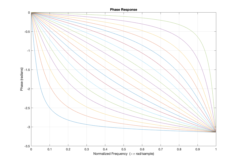
\[H_r(z) = \Lambda_0(z)A(z)^r, \textbf{ } r = 0,1,....\]

Here, the authors do not go into much detail about what is meant by this and what $H_r$ refers to. I went through some of their earlier papers and learned that this expression is the z-transform of an order-\(r\) Laguerre sequence. Laguerre sequences are kernels on which one can expand signals through a process known as the Laguerre transform. They form a complete orthonormal set in the space \(l^2\) of finite energy causal sequences for any fixed value of the parameter \(b\) such that \(-1<b<1.\) These so-called Laguerre warping maps are shown in Figure 1.

An implementation of the above Laguerre transform occurrence is performed by time-reversing the signal, filtering by the orthogonalizing factor \(\Lambda_0\) and evaluating the iterated convolution with the first order all-pass impulse response at time lag 0. This structure is shown in Figure 2.

Figure 1. Family of Laguerre warping maps for parameter \(b\) varying from \(-0.9, -0.8, ..., 0.8, 0.9.\) These are equivalent to the negative of the phase response of a first-order all-pass filter.

Figure 2. Digital structure implementing the Laguerre transform.

Time-varying frequency warping

Time-varying frequency warping can simply be considered as a generalization of the transform described in the previous section to the $n$-order case. Consider a sequence \(\psi_n[k]\) onto which we will project our discrete-time signal $x[k]$. If \(\psi_n[k]\) is characterized by an order \(n\) all-pass filter, it’s z-transform can be written as

\[\phi_n(z) = \begin{cases} 1 & \text{if $n=0$} \\ \prod_{k=1}^n \frac{z^{-1}-b_k}{1-b_kz^{-1}} & \text{if $n>0$} \end{cases}\]

which corresponds to a frequency dependent delay

\[\phi_n(\omega) = e^{-\Omega_n(\omega)}\]

where \(\Omega_n(\omega) = \sum_{k=1}^n \theta_k(\omega),\)

with

\[\omega_k(\omega) = -\text{arg}A_k(e^{j\omega}) = \omega + 2\tan^{-1}\left[\frac{b_k\sin\omega}{1-b_k\cos\omega}\right].\]

This structure, known as a sampled dispersive delay line, is closely related to the time-invariant case and is shown in Figure 3.

Figure 3. Time-varying frequency warping structure based on a sampled dispersive delay line.

An application: Demodulation of flute vibrato

The authors of the paper showed several applications of time-varying frequency warping but little to no detail for how they were implemented was given. The applications shown included pitch modulation removal (which we’ll attempt to recreate here), signal detection (if buried in a high level of noise), pitch modulation effects, chorusing, flanging, phasing, morphing, and pitch-shifting.

Consider a recording of a flute which has unwanted vibrato. One can “regularize" the sound (e.g. remove the vibrato) by performing time-varying frequency warping against the vibrato. The structures shown in Figures 2 and 3 were implemented in MATLAB 2019B for this purpose. The flute recording was obtained from freesound.org.

Fundamental frequency estimation was performed on the recording by MATLAB’s [pitch]{.smallcaps} function. The method used is called Pitch Estimation Filter and is described in [6]. This $f_0$ estimation returns an array of frequency values with a length that is roughly \(0.7\%\) of the length of the input signal. The central piece in an implementation of time-varying frequency warping involves the evolution of the parameter $b$ on the interval \((-1,1)\). The size of the array \(b\) that describes its time evolution is roughly the length \(L\) of the input signal. Accordingly, I extrapolated the \(f_0\) data onto an array that had a length equivalent to that of \(L\) using MATLAB’s [interp1]{.smallcaps} function. Then, I rescaled this array to be centered around zero and having a range contained on the interval \((-1,1)\).

The most difficult part of my method was determining the scale to which I should resize this array. After much trial and error, I found that the scale that achieves the best demodulation was [-0.5,0.5]. Then, to keep improving on the demodulation, I iterated the algorithm several times, using the output of the previous run as the input. This drastically improved the results. The \(f_0\) estimation of the truncated (to improve calculation time) unwarped signal is shown in Figure 4. The change in \(f_0, \Delta f_0 = 11.8\) Hz. The warped version of the same signal is shown in Figure 5 with \(\Delta f_0 = 2.73\) Hz. I am confident that my algorithm can be improved upon even more to achieve a \(\Delta f_0 < 1\) Hz.

Figure 4. \(f_0\) estimation of truncated unwarped flute signal. Notice the vibrato contour. Range of \(f_0\): 11.8 Hz.

Figure 5. \(f_0\) estimation of demodulated warped flute signal. Notice y-axis scale. Range of \(f_0\): 2.73 Hz.

Conclusions

In conclusion, time-varying frequency warping is ubiquitous in the processing of musical signals due to its high level of flexibility. In this paper, we have explored the work of Evangelista and Cavaliere [1] who introduced an efficient algorithm to do this based on an expansion over biorthogonal sets generalizing the discrete Laguerre basis. We then showed an implementation and application to demodulation of a flute with vibrato.

I learned quite a bit from this project and hope to continue exploring frequency warping in the context of music. In particular, I am interested in its applications for physical modeling of acoustic instruments that show some inharmonicity, such as the piano. Furthermore, I am interested in exploring a real-time implementation of this in Max/MSP. I began to create a Max patch but quickly found that it was far beyond the scope of this project. The idea is to perform a “short-time Laguerre transform" on audio buffers and be able to change the parameter $b$ in real-time. This could someday be a very useful tool for electroacoustic composers and performers.

References

[1] Evangelista, G., & Cavaliere, S. (2001). Audio Effects Based on Biorthogonal Time-Varying Frequency Warping. EURASIP Journal on Advances in Signal Processing, 2001(1), 289319. doi:10.1155/S1110865701000130

[2] Evangelista, G. (2008, 12-14 March 2008). Modified phase vocoder scheme for dynamic frequency warping. Paper presented at the 2008 3rd International Symposium on Communications, Control and Signal Processing.

[3] Broome, P. W. (1965). Discrete Orthonormal Sequences. J. ACM, 12(2), 151–168. doi:10.1145/321264.321265

[4] Oppenheim, A. V., & Johnson, D. H. (1972). Discrete representation of signals. Proceedings of the IEEE, 60(6), 681-691.

[5] Baraniuk, R. G., & Jones, D. L. (1995). Unitary equivalence: a new twist on signal processing. IEEE Transactions on Signal Processing, 43(10), 2269-2282.

[6] Gonzalez, S., & Brookes, M. (2011, 29 Aug.-2 Sept. 2011). A Pitch Estimation Filter robust to high levels of noise (PEFAC). Paper presented at the 2011 19th European Signal Processing Conference.

[7] Evangelista, G. (2011). Time and Frequency-Warping Musical Signals. In U. Zolzer (Ed.), DAFX: Digital Audio Effects (pp. 447-471).

---