Extending Optimized Dual Gabor Windows to the Nonstationary Case in Musical Signals

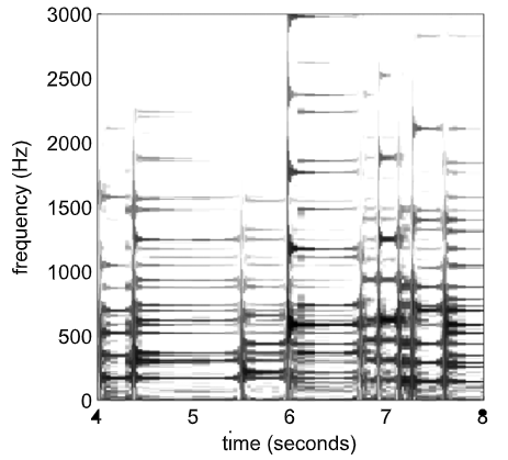
Figure 1. Nonstationary Gabor transform of a snippet of a solo Herbie Hancock recording. Taken from [1].

Introduction

In audio signal processing, a wealth of research is devoted to finding methods that achieve flexible tilings of the time-frequency plane. By projecting signals onto time-frequency atoms of the form \(g_{\tau,\omega},\) one can perform sparse atomic decomposition to analyze and possibly resynthesize signals. The most popular of these methods is the short-time Fourier transform, a highly redundant transform that involves translates and modulations of a single window function. Gabor analysis [3] generalizes short-time Fourier methods by super-imposing a grid on the time-frequency plane with fixed resolution. The Gabor transform of a discrete-time signal \(f\) is then projections \(⟨f,g_{\tau,\omega} ⟩\) of \(f\) onto atoms \(g_{\tau,\omega}\) where \(g_{\tau,\omega}\) are translated and modulated versions of single window function \(g\): \(g_{\tau,\omega}[t] = g[t-\tau]e^{2\pi jt\omega}.\)

In order to achieve perfect reconstruction from a signal analyzed using a time-frequency transform, one needs to use a dual window that allows for such reconstruction. A window and its dual that allow for perfect reconstruction are henceforth referred to as a PR pair. The most common choice for a dual window that constitutes a PR pair is the canonical dual window. This window is readily available via a pseudoinverse of the analysis operator, is computationally efficient, and minimizes the \(l^2\)-norm. Indeed, the canonical dual is used in [1] for efficient reconstruction from the nonstationary Gabor transform.

However, as pointed out in [2], the canonical dual might lack properties that are desired in a given context and is therefore not optimal. For example, if we are interested in high quality processing, we need good time-frequency concentration, a feature not provided by the canonical dual. A better choice might be to choose a dual window that is optimized for good time-frequency concentration. Accordingly, Perraudin et al. [2] proposed a framework to compute optimized dual windows given criteria that describe various preferable TF characteristics. They use tools from modern convex optimization to search a space of functions equal to the solution set of the Wexler-Raz equations, thus allowing for PR. A number of numerical experiments were carried out to optimize various conditions. In the present paper, we will interpret those results in the context of nonstationary musical signals.

It should be noted that optimized dual windows are only useful in the case of modified Gabor coefficients, since all dual windows perform PR from unmodified coefficients. Thus, we will use basic frame multipliers (also known as Gabor filters) to remove time-frequency components from a signal through modification of the Gabor coefficients.

The rest of this paper is organized as follows. We fix notation and review preliminary results from Gabor and frame theory in Section 2. In Section 3, we will extend these ideas to the nonstationary case with time-frequency resolution changing over time or frequency. Section 4 will briefly introduce the concept of frame multipliers for performing source separation of time-frequency components. In Section 5, we will review the results of [2] for optimizing dual Gabor windows. Section 6 will combine the ideas from the previous sections in the context of the removal of a time-frequency component from a musical signal. We conclude, in Section 7, with a summary and reflections on our work.

Preliminaries

In this paper, we consider sampled functions, i.e. sequences \(f\) in \(l^2(\mathbb{Z})\). The smallest closed interval containing all nonzero values of \(f\) will be referred to as its support, denoted by \(\text{supp}(f).\) As Gabor analysis concerns itself with translated and modulated versions of a single window function \(g\), we will introduce the following translation and modulation operators to ease notation:

\[\textbf{T}_nf[l] = f[l-n] \text{ and } \textbf{M}_\omega f[l] = f[l]e^{2\pi j \omega l},\]

for \(f \in l^2(\mathbb{Z}), l, n \in \mathbb{Z},\) and normalized frequency \(\omega \in [0,1).\)

Gabor systems, frames, and dual windows

Given a non-zero window function \(g\), a hop size \(a\), and a number of frequency bins \(M,\) a Gabor system is defined as the set of time-frequency shifts of \(g\)

\[\mathcal{G}(g,a,M) := (g_{m,n} = \textbf{M}_{m/M}\textbf{T}_{na}g)_{n\in \mathbb{Z},\textbf{ } m = 0,1,...,M-1}.\]

Figure 1 shows a basic discretization of the TF plane using the Gabor system \(\mathcal{G}(g,3,4)\). In practice, the length of the window \(g\) will overlap some amount with adjacent windows, allowing for PR. For some signal \(f \in l^2(\mathbb{Z}\), the Gabor coefficients (Gabor analysis) with respect to \(\mathcal{G}(g,a,M)\) are given by

\[(\textbf{G}f)[m+nM] = ⟨f,g_{m,n}⟩ = \sum_{l\in \mathbb{Z}} f[l]\overline{g_{m,n}[l]},\]

with the analysis operator \(\textbf{G}\) given by the infinite matrix \(\textbf{G}[m+nM,l] := \textbf{G}_{g,a,M}[m+nM,l]:= \overline{g_{m,n}[l]}.\)

A basic example of a TF-plane discretization using the Gabor system \(\mathcal{G}(g,3,4)\). The arrows on the time axis denote the hop size \(a = 3\) and the arrows on the frequency axis denote the number of channels \(M = 4.\)

Gabor synthesis of a coefficient sequence \(c \in l^2(\mathbb{Z})\) with respect to \(\mathcal{G}(g,a,M)\) is performed by

\[f_{syn}[l] = (\textbf{G*}c)[l] = \sum_{n \in \mathbb{Z}}\sum_{m=0}^{M-1}c[m+nM]g_{m,n}[l],\]

where \(\textbf{G*}\) denotes the conjugate transpose of \(\textbf{G}.\) A Gabor transform with \(a=1\) and \(M=L\), where \(L\) is the length of the signal, is also known as the short-time Fourier transform (STFT).

In order to perform inversion using the synthesis operator \(\textbf{G*},\) we require that the Gabor system \(\mathcal{G}(g,a,M)\) forms a stable, overcomplete system satisfying

\[A||f||^2_2 \leq ||\textbf{G}f||^2_2 \leq B||f||^2_2, \text{ for all } f\in l^2(\mathbb{Z}),\]

for some \(0 < A \leq B < \infty\). Then, it is called a Gabor frame. In that case, every signal \(f \in l^2(\mathbb{Z})\) can be written as

\[f = \textbf{G*}_{g,a,M}c\]

for some coefficient sequence \(c \in l^2(\mathbb{Z}).\) If \(A = B\) is a valid choice, it is called a tight frame. In that case, \(h = g/A = g/B\) constitutes a dual window. The frame property guarantees the existence of a dual Gabor frame \(\mathcal{G}(h,a,M)\) such that

\[f = \textbf{G*}_{h,a,M}(\textbf{G}_{g,a,M}f) = \textbf{G*}_{g,a,M}(\textbf{G}_{h,a,M}f)\]

holds for all \(f \in l^2(\mathbb{Z}).\) Thus, the coefficient sequence \(c\) in the above equation can be chosen to be the Gabor coefficients with respect to \(\mathcal{G}(h,a,M)\).

Construction of nonstationary Gabor frames

Resolution changing over time

The setting of nonstationary Gabor frames allows for changing (adaptive) windows in different time positions. Then, for each time position, we build atoms by regular frequency modulation. Using a set of functions \(g_n\) for \(n\in \mathbb{Z}\) in \(l^2(\mathbb{R})\) and frequency sampling step \(b_n,\) we define atoms of the form \(g_{m,n}[l] = \textbf{M}_{mb_n/M}g_n[l] = g_n[l]e^{2\pi j mb_nl}\)

for \(m = 0,1,...,M-1\) and \(n\in \mathbb{Z}.\) The only difference between this and standard Gabor theory is that now we can vary the window \(g_n\) at each time-step \(a_n.\) Therefore, the time-frequency lattice becomes regular over frequency at each temporal position but irregular over time.

Example of a sampling grid for the nonstationary Gabor transform with a) TF resolution changing over time and b) TF resolution changing over frequency.

Resolution changing over frequency

A logical continuation is to irregularly sample the frequency axis using windows that feature adaptive bandwidth. Then, sampling is regular over the time axis. To do this, we’ll introduce a family of functions \(h_m\) for \(m \in 0,1,...,M-1$ in $l^2(\mathbb{R})\) and define atoms of the form

\[h_{m,n}[l] = \textbf{T}_{na_m}h_m = h_m[l - na_m]\]

for \(n\in \mathbb{Z}\). In practice, \(h_m\) will be chosen as a well localized band-pass function with center frequency \(b_n\).

Gabor multipliers

Gabor multipliers are linear operators on sequences \(f \in l^2(\mathbb{Z})\) defined by pointwise multiplication with a TF transfer function called a Gabor mask, in the Gabor coefficients domain. If we denote the Gabor mask by \(\textbf{u}\) and the multiplier operator by \(\textbf{U}\), then the Gabor multiplier associated to the Gabor system \(\mathcal{G}(g,a,M)\) is defined by \(\textbf{U}_\textbf{u} = \textbf{G*}\textbf{u}\textbf{G}\), where \(\textbf{G}\) is the analysis operator as described in Section 2. Applied to a signal \(f,\) we have

\[\textbf{U}_\textbf{u}f = \sum_{m,n}\textbf{u}[m,n]⟨f, g_{m,n}⟩g_{m,n}.\]

Gabor multipliers have been studied extensively in [4], [5], and, more recently, in [6]. Their properties are not particularly relevant to the current investigation but the curious reader is invited to review the references above for more information.

Dual Gabor frames beyond the canonical dual

In this section, we will review some results from [2] and investigate their relevance to the current investigation. As mentioned previously, Gabor frames allow for a redundant representation of a signal and are therefore necessary for perfect reconstruction. Their use allows for an infinite number of dual frames, frames used for resynthesizing a signal from the Gabor coefficients (analysis). In the literature of Gabor theory, the dual window known as the canonical dual is, by far, the most widely used. However, Perraudin et al. [2] argue that the canonical dual might lack desirable properties, e.g. good time-frequency concentration, small support, or smoothness. Therefore, it is useful to search the entire set of dual windows for one that best fits a given context.

The Wexler-Raz Equations

In 1990, Wexler and Raz [7] showed that if the Gabor system \(\mathcal{G}(g,a,M)\) is redundant, then the dual window \(h\in l^2(\mathbb{Z})\) is not unique. Rather, the space of dual windows equals the solution set of the so-called Wexler-Raz equations that characterize the dual Gabor windows for \(\mathcal{G}(g,a,M)\). They are given by

\(\frac{M}{a}⟨h,g[\cdot - nM]e^{2\pi jm\cdot /a}⟩ = \delta[n]\delta[m]\)\(\text{ or }\)\(\textbf{G}_{g,M,a}h = [a/M,0,0,...]^T\)

for \(m=0,...,a-1, n\in \mathbb{Z}\). Here, \(\delta\) denotes the Kronecker delta and \(\textbf{G}_{g,M,a}\) denotes the analysis operator of the Gabor system with window \(g\), hop size \(M\), and number of channels \(a\). Note that, while \(\textbf{G}_{g,a,M}\) is overcomplete, \(\textbf{G}_{g,M,a}\) is underdetermined and admits infinitely many solutions.

Convex Optimization

In mathematics and computer science, an optimization problem is an attempt to find the best solution among all feasible solutions. In order to determine what constitutes the best solution, an objective function is invoked. Often, one wants to minimize this objective function subject to certain constraints. If the objective function and the search space are convex, the problem is known as a convex optimization problem.

In order to use convex optimization to design dual Gabor windows, we will consider convex optimization problems of the form

\[\mathop{\mathrm{minimize}}_{x\in \mathbb{R}^L}\sum_{i=1}^K f_i(x)\]

where the \(f_i\) are convex functions that promote certain features in the solution. These functions are also called priors. Many algorithms exist to solve this type of optimization problem. The authors of [2] chose a method called proximal splitting that only require the \(f_i\) to be lower semi-continuous, convex and proper functions, thus allowing to increase the design freedom. More information and convergence results can be found in [8].

Design of optimal dual windows

The solution set of aforementioned Wexler-Raz equations becomes the search space for our optimization problem. Additionally, we may want to impose a support constraint on the search space. That is, only allow the search space to be the set of all functions in \(l^2(\mathbb{Z})\) supported on some interval \(I_h\). Then, we can reformulate our convex optimization problem as

\[\mathop{\mathrm{arg min}}_{x\in \mathcal{C}_{\text{dual}}\cap \mathcal{C}_{\text{supp}}} \sum_{i=1}^K f_i(x)\]

where \(\mathcal{C}_{\text{dual}}\) is the set of dual windows allowed by the Wexler-Raz equations, \(\mathcal{C}_{\text{supp}}\) is the set of functions in \(l^2(\mathbb{Z})\) supported on \(I_h\) and \(f_i\) are priors that promote certain features in the solution. In practice, each \(f_i\) is weighted by a regularization parameter \(\lambda_i > 0\). Table 1 contains a list of relevant priors along with their effect on the signal and time complexity.

                                                   Table of important priors \(f_i\) and their effect on the signal.

Removing TF components in musical signals

Recall that optimized dual windows are only useful in the case of modified Gabor coefficients. Accordingly, let’s say we want to remove a time-frequency component from a signal. One approach would be to take the nonstationary Gabor transform, apply a Gabor multiplier to the analysis coefficients, and resynthesize with a dual window. For the current investigation, we will use a recording of glockenspiel. The nonstationary Gabor transform of the signal is shown in Figure 4 along with a zoomed in version of the same transform. The glockenspiel is useful for our purposes due to its strong transient attack followed by decaying sinusoidal components. All computations were made with the NonStationary Gabor Toolbox and the Large Time-Frequency Analysis Toolbox (LTFAT) on MATLAB 2019B.

a. Nonstationary Gabor transform of a glockenspiel (computed with Hann windows of varying length) with a b. zoomed-in version on the lower frequencies of five sequential notes of the same pitch.

Let’s say we would like to remove the transient part of the third (middle) of the five notes shown in Figure 4b. The resulting unachievable target spectrogram is shown in Figure 5.

Unachievable 'oracle' nonstationary Gabor transform of glockenspiel signal with transient part of third note removed.

In order to achieve this, we will use a basic Gabor multiplier and apply it to the coefficients. The Gabor mask used simply zeroed out all the coefficients in the time-span of the transient. Reconstruction was performed with the canonical dual window and results are shown in Figure 6. Notice the smearing in the region of interest. A root mean square reconstruction error was computed by calculating the \(l_2\) norm of the original signal \(s\) minus the reconstructed signal \(s_r\) then normalized by the \(l_2\) norm of \(s\).

\[\text{RMS}(s,s_r) = \sqrt{\frac{\sum_{k=0}^{L-1}|s[k] - s_r[k]|^2}{\sum_{k=0}^{L-1}|s[k]|^2}}\]

Thus, we will conduct a series of experiments through optimizing dual Gabor windows to reduce this smearing. The results are depicted in Figures 7-10.

Reconstruction using canonical dual window. Notice smearing in region of interest. Relative error of reconstruction: 1.165428e-01

Reconstruction by optimizing variance in frequency. Notice smearing in region of interest. Relative error of reconstruction: 1.177556e-01

Reconstruction by optimizing smoothing parameter in frequency. Relative error of reconstruction: 1.161806e-01

Reconstruction by optimizing variance in time. Relative error of reconstruction: 1.115359e-01

Reconstruction by optimizing smoothing parameter in time. Relative error of reconstruction: 1.525052e-01

Conclusions

We have shown a method for removing time-frequency components through use of a Gabor multiplier and optimization of Gabor dual windows in the nonstationary Gabor transform. These results show that, while no optimization parameter could truly eliminate the smearing effect, the variance in time parameter had the smallest relative error of reconstruction.

The general methods proposed in this paper could be extended to many sorts of problems including denoising and source separation. I am very fascinated by the potential of the NSGT and will no doubt continue to read about it and investigate further applications. I also look forward to learning more about Gabor multipliers and various ways they can be computed.

References

[1] Balazs, P., Dörfler, M., Jaillet, F., Holighaus, N., & Velasco, G. (2011). Theory, implementation and applications of nonstationary Gabor frames. Journal of Computational and Applied Mathematics, 236(6), 1481-1496. doi:https://doi.org/10.1016/j.cam.2011.09.011

[2] Perraudin, N., Holighaus, N., Søndergaard, P. L., & Balazs, P. (2018). Designing Gabor windows using convex optimization. Applied Mathematics and Computation, 330, 266-287. doi:https://doi.org/10.1016/j.amc.2018.01.035

[3] Feichtinger, H., & Zimmermann, G. (1998). Gabor Analysis and Algorithms. In (pp. 123-170).

[4] Doerfler, M. (2002). Gabor analysis for a class of signals called music.

[5] Feichtinger, H., & Nowak, K. (2002). A First Survey of Gabor Multipliers. doi:10.1007/978-1-4612-0133-5_5

[6] Krémé, A. M., Emiya, V., Chaux, C., & Torresani, B. (2020). Filtering out time-frequency areas using Gabor mulipliers. Paper presented at the ICASSP: 45th International Conference on Acoustics, Speech, and Signal Processing, Barcelone, Spain. https://hal.archives-ouvertes.fr/hal-02456153

[7] Wexler, J., & Raz, S. (1990). Discrete Gabor expansions. Signal Processing, 21(3), 207-220. doi:https://doi.org/10.1016/0165-1684(90)90087-F

[8] Rockafellar, R. T. (1976). Monotone Operators and the Proximal Point Algorithm. SIAM Journal on Control and Optimization, 14(5), 877-898. doi:10.1137/0314056

---